| mpg | cyl | disp | hp | drat | wt | qsec | vs | am | gear | carb | |
|---|---|---|---|---|---|---|---|---|---|---|---|
| Mazda RX4 | 21.0 | 6 | 160.0 | 110 | 3.90 | 2.620 | 16.46 | 0 | 1 | 4 | 4 |
| Mazda RX4 Wag | 21.0 | 6 | 160.0 | 110 | 3.90 | 2.875 | 17.02 | 0 | 1 | 4 | 4 |
| Datsun 710 | 22.8 | 4 | 108.0 | 93 | 3.85 | 2.320 | 18.61 | 1 | 1 | 4 | 1 |
| Hornet 4 Drive | 21.4 | 6 | 258.0 | 110 | 3.08 | 3.215 | 19.44 | 1 | 0 | 3 | 1 |
| Hornet Sportabout | 18.7 | 8 | 360.0 | 175 | 3.15 | 3.440 | 17.02 | 0 | 0 | 3 | 2 |
| Valiant | 18.1 | 6 | 225.0 | 105 | 2.76 | 3.460 | 20.22 | 1 | 0 | 3 | 1 |
| Duster 360 | 14.3 | 8 | 360.0 | 245 | 3.21 | 3.570 | 15.84 | 0 | 0 | 3 | 4 |
| Merc 240D | 24.4 | 4 | 146.7 | 62 | 3.69 | 3.190 | 20.00 | 1 | 0 | 4 | 2 |
| Merc 230 | 22.8 | 4 | 140.8 | 95 | 3.92 | 3.150 | 22.90 | 1 | 0 | 4 | 2 |
| Merc 280 | 19.2 | 6 | 167.6 | 123 | 3.92 | 3.440 | 18.30 | 1 | 0 | 4 | 4 |
| Merc 280C | 17.8 | 6 | 167.6 | 123 | 3.92 | 3.440 | 18.90 | 1 | 0 | 4 | 4 |
| Merc 450SE | 16.4 | 8 | 275.8 | 180 | 3.07 | 4.070 | 17.40 | 0 | 0 | 3 | 3 |
| Merc 450SL | 17.3 | 8 | 275.8 | 180 | 3.07 | 3.730 | 17.60 | 0 | 0 | 3 | 3 |
| Merc 450SLC | 15.2 | 8 | 275.8 | 180 | 3.07 | 3.780 | 18.00 | 0 | 0 | 3 | 3 |
| Cadillac Fleetwood | 10.4 | 8 | 472.0 | 205 | 2.93 | 5.250 | 17.98 | 0 | 0 | 3 | 4 |
| Lincoln Continental | 10.4 | 8 | 460.0 | 215 | 3.00 | 5.424 | 17.82 | 0 | 0 | 3 | 4 |
| Chrysler Imperial | 14.7 | 8 | 440.0 | 230 | 3.23 | 5.345 | 17.42 | 0 | 0 | 3 | 4 |
| Fiat 128 | 32.4 | 4 | 78.7 | 66 | 4.08 | 2.200 | 19.47 | 1 | 1 | 4 | 1 |
| Honda Civic | 30.4 | 4 | 75.7 | 52 | 4.93 | 1.615 | 18.52 | 1 | 1 | 4 | 2 |
| Toyota Corolla | 33.9 | 4 | 71.1 | 65 | 4.22 | 1.835 | 19.90 | 1 | 1 | 4 | 1 |
| Toyota Corona | 21.5 | 4 | 120.1 | 97 | 3.70 | 2.465 | 20.01 | 1 | 0 | 3 | 1 |
| Dodge Challenger | 15.5 | 8 | 318.0 | 150 | 2.76 | 3.520 | 16.87 | 0 | 0 | 3 | 2 |
| AMC Javelin | 15.2 | 8 | 304.0 | 150 | 3.15 | 3.435 | 17.30 | 0 | 0 | 3 | 2 |
| Camaro Z28 | 13.3 | 8 | 350.0 | 245 | 3.73 | 3.840 | 15.41 | 0 | 0 | 3 | 4 |
| Pontiac Firebird | 19.2 | 8 | 400.0 | 175 | 3.08 | 3.845 | 17.05 | 0 | 0 | 3 | 2 |
| Fiat X1-9 | 27.3 | 4 | 79.0 | 66 | 4.08 | 1.935 | 18.90 | 1 | 1 | 4 | 1 |
| Porsche 914-2 | 26.0 | 4 | 120.3 | 91 | 4.43 | 2.140 | 16.70 | 0 | 1 | 5 | 2 |
| Lotus Europa | 30.4 | 4 | 95.1 | 113 | 3.77 | 1.513 | 16.90 | 1 | 1 | 5 | 2 |
| Ford Pantera L | 15.8 | 8 | 351.0 | 264 | 4.22 | 3.170 | 14.50 | 0 | 1 | 5 | 4 |
| Ferrari Dino | 19.7 | 6 | 145.0 | 175 | 3.62 | 2.770 | 15.50 | 0 | 1 | 5 | 6 |
| Maserati Bora | 15.0 | 8 | 301.0 | 335 | 3.54 | 3.570 | 14.60 | 0 | 1 | 5 | 8 |
| Volvo 142E | 21.4 | 4 | 121.0 | 109 | 4.11 | 2.780 | 18.60 | 1 | 1 | 4 | 2 |
Computation
Markdown table
| City     | Country |
|----------|---------|
| Mannheim | Germany |
| Paris    | France  |
| Tokyo | Japan || City | Country |
|---|---|
| Mannheim | Germany |
| Paris | France |
| Tokyo | Japan |
Exercise
Create a Tic Tac Toe field and play a game with yourself
| X | X | O |
|---|---|---|
| O | O | X |
| X | O | O |
Code chunks
Literate programming: mixing a document formatting language and a programming language.
Code chunks are snippets of programming language to do the “mixing”. You can insert a code chunk in a Quarto document with (at least) three backticks.
```r
x <- "Hello World!"
message(x)
```

```python
x = "Hello World!"
print(x)
```

```c
int main() {
    printf("Hello World!");
    return 0;
}
```
Exercise 1
Copy and paste the R code chunk into a Quarto document and render it. Tell us what’s the output.
Exercise 2 (Optional)
This workshop is really not about R, but we still need to use R. If you don’t know (enough) R, try to familiarize yourself with the following. If you know all of them, congratulations you know enough R to survive this session!
1 + 2 - 3 * 4 / 3
x <- "hello world"
x
## message
message(x)
## mtcars is a built-in dataset. The data structure is called data frame
mtcars
## simple functions
nrow(mtcars)
head(mtcars)
## basic viz
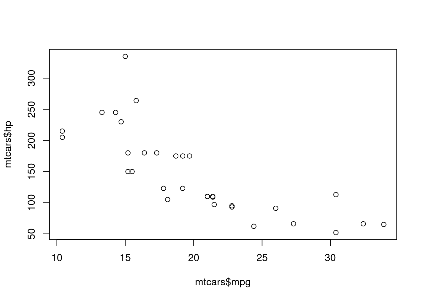
plot(mtcars$mpg, mtcars$hp)
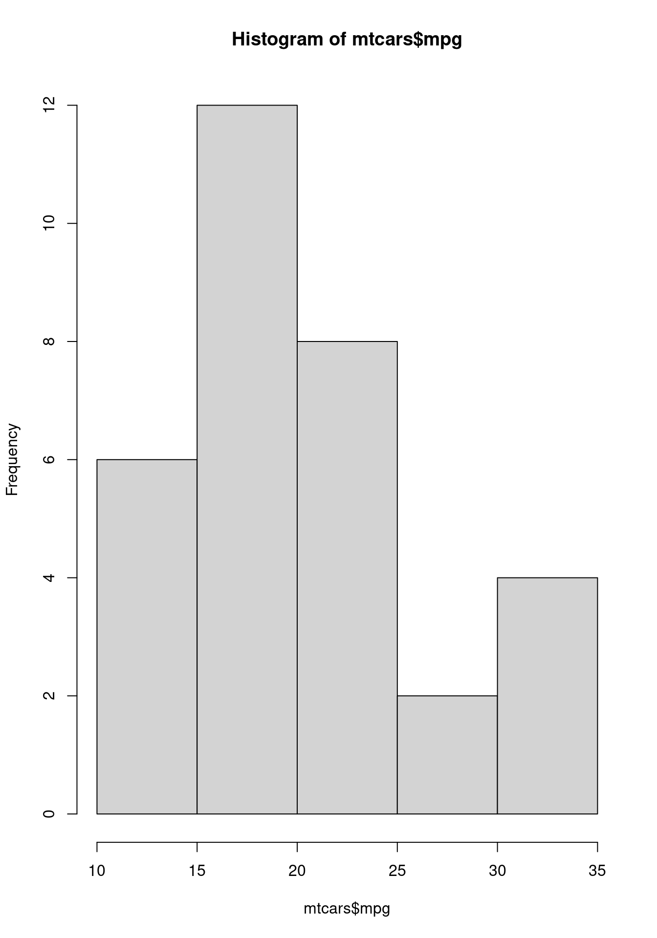
hist(mtcars$mpg)
## installing external packages
install.packages("knitr")
## You can either call the package by `library`
library(knitr)
kable
## or the namespace operator ::
knitr::kable
## read some data, if your csv file is called hello.csv
x <- read.csv("hello.csv")
## get help
?read.csvComputation Option 1: Executable Code chunk
The way to insert a code chink in the previous exercise does not involve code execution. Therefore, Quarto will only format the code, e.g. add syntax highlight.
To make the code executable, wrap r with a pair of curly.
```{r}
x <- "Hello World!"
message(x)
```
Exercise 1
Copy and paste the R code chunk into a Quarto document and render it. Tell us what’s the output.
```{r}
x <- "Hello World!"
message(x)
```
Exercise 2
Create a code chunk in a Quarto document to calculate the area of a circle with radius = 10 (hints: pi). Render it.
Computation Option 2: Inline R code (knitr)
Another way to invoke code execution is to use inline code: `r `
## Mathematics

I don't know the answer of 1 + 1 equals to 2.
When to use inline?
For quick and dirty generation of one number in a paragraph, e.g. number of observations, calculation of mean. Otherwise, use code chunk.
Exercise 1:
Convert the above area calculation to inline R code.
Exercise 2:
Write inline R code to display the following sentence (hints: nrow):
There are 32 observations in the data frame mtcars.
Full circle
Some R functions generate Markdown code.
mtcars
knitr::kable(mtcars)
Exercise
Display the content of mtcars as a table in a Quarto document like the following:
Figures
```{r}
hist(mtcars$mpg)
```
Exercise
Display a scatter plot in a Quarto document like the following:
Execution Options
You can control how the code is executed with execution options
Output options (knitr)
```{r}
#| echo: false
knitr::kable(mtcars)
```
There are
eval(evaluate the code chunk or not)echo(include the source code or not in the output)output(include the execution result in the output or not:true,false,asis)warning(include warnings in the output)error(include errors in the output)include(include: falsesuppresses all output, useful for reading data or loading packages)
Exercise
Read this file and make Quarto display the following:
There are 344 observations in the file penguins_raw.csv and the first few rows look like so:
| studyName | Sample.Number | Species | Region | Island | Stage | Individual.ID | Clutch.Completion | Date.Egg | Culmen.Length..mm. | Culmen.Depth..mm. | Flipper.Length..mm. | Body.Mass..g. | Sex | Delta.15.N..o.oo. | Delta.13.C..o.oo. | Comments |
|---|---|---|---|---|---|---|---|---|---|---|---|---|---|---|---|---|
| PAL0708 | 1 | Adelie Penguin (Pygoscelis adeliae) | Anvers | Torgersen | Adult, 1 Egg Stage | N1A1 | Yes | 2007-11-11 | 39.1 | 18.7 | 181 | 3750 | MALE | NA | NA | Not enough blood for isotopes. |
| PAL0708 | 2 | Adelie Penguin (Pygoscelis adeliae) | Anvers | Torgersen | Adult, 1 Egg Stage | N1A2 | Yes | 2007-11-11 | 39.5 | 17.4 | 186 | 3800 | FEMALE | 8.94956 | -24.69454 | NA |
| PAL0708 | 3 | Adelie Penguin (Pygoscelis adeliae) | Anvers | Torgersen | Adult, 1 Egg Stage | N2A1 | Yes | 2007-11-16 | 40.3 | 18.0 | 195 | 3250 | FEMALE | 8.36821 | -25.33302 | NA |
| PAL0708 | 4 | Adelie Penguin (Pygoscelis adeliae) | Anvers | Torgersen | Adult, 1 Egg Stage | N2A2 | Yes | 2007-11-16 | NA | NA | NA | NA | NA | NA | NA | Adult not sampled. |
| PAL0708 | 5 | Adelie Penguin (Pygoscelis adeliae) | Anvers | Torgersen | Adult, 1 Egg Stage | N3A1 | Yes | 2007-11-16 | 36.7 | 19.3 | 193 | 3450 | FEMALE | 8.76651 | -25.32426 | NA |
| PAL0708 | 6 | Adelie Penguin (Pygoscelis adeliae) | Anvers | Torgersen | Adult, 1 Egg Stage | N3A2 | Yes | 2007-11-16 | 39.3 | 20.6 | 190 | 3650 | MALE | 8.66496 | -25.29805 | NA |
Figure Options (knitr)
There are:
fig-widthfig-heightfig-capfig-altfig-alignfig-dpi
An example to play around
```{r}
#| fig-cap: "A random histogram"
#| fig-height: 10
#| fig-align: right
#| echo: false
hist(mtcars$mpg)
```
Best practices
Label your chunk
It does nothing apparently. You will know why it is important tomorrow. All labels must be unique.
```{r}
#| label: mtcars_listing
#| echo: false
knitr::kable(mtcars)
```
(Not) cache
You can cache the computational result of a chunk (save the result as a file. When the Quarto file is being rendered again, the cached result is used instead of doing the computation again). It’s best to use it with a labeled code chunk. In general, it is not recommended for a reproducible scientific workflow. Use it unless you know what you are doing.
```{r}
#| label: mtcars_listing
#| echo: false
#| cache: true
knitr::kable(mtcars)
```
Engines
R code inside a Quarto document is handled by the computational engine knitr. You might want to use another computational engine if R is not your thing. For example, Python code is handled by Jupyter. In a mix language environment, you might need reticulate.
```{python}
## This is all the Python I know

def fib(n):
    a, b = 0, 1
    for _ in range(n):
        yield a
        a, b = b, a + b
list(fib(5))
```
## This is all the Python I know
def fib(n):
a, b = 0, 1
for _ in range(n):
yield a
a, b = b, a + b
list(fib(5))[0, 1, 1, 2, 3]Debrief
Q: How to display table caption?
A:
With computation
```{r}
#| echo: false
#| tbl-cap: "Just a few rows"
#| tbl-cap-location: bottom
#| label: headmtcars
knitr::kable(head(mtcars))
```| mpg | cyl | disp | hp | drat | wt | qsec | vs | am | gear | carb | |
|---|---|---|---|---|---|---|---|---|---|---|---|
| Mazda RX4 | 21.0 | 6 | 160 | 110 | 3.90 | 2.620 | 16.46 | 0 | 1 | 4 | 4 |
| Mazda RX4 Wag | 21.0 | 6 | 160 | 110 | 3.90 | 2.875 | 17.02 | 0 | 1 | 4 | 4 |
| Datsun 710 | 22.8 | 4 | 108 | 93 | 3.85 | 2.320 | 18.61 | 1 | 1 | 4 | 1 |
| Hornet 4 Drive | 21.4 | 6 | 258 | 110 | 3.08 | 3.215 | 19.44 | 1 | 0 | 3 | 1 |
| Hornet Sportabout | 18.7 | 8 | 360 | 175 | 3.15 | 3.440 | 17.02 | 0 | 0 | 3 | 2 |
| Valiant | 18.1 | 6 | 225 | 105 | 2.76 | 3.460 | 20.22 | 1 | 0 | 3 | 1 |
Without computation
| City     | Country |
|----------|---------|
| Mannheim | Germany |
| Paris    | France  |
| Tokyo    | Japan   |

: List of cities
| City | Country |
|---|---|
| Mannheim | Germany |
| Paris | France |
| Tokyo | Japan |
Q: I’ve heard that the knitr::kable call is not necessary.
A: You are right. Quarto (or the rendering engine: knitr) can convert all data.frame objects to Markdown tables using the df-print document option. You will learn about document options a.k.a. YAML Front Matter in the next session.
Q: Does interactive viz work?
A: Oui.
```{r}
#| echo: false
#| fig-height: 2
#| fig-width: 5
#| label: ggplotly_demo
library(ggplot2)
library(plotly)
fig <- ggplot(mtcars, aes(wt, mpg)) + geom_point()
ggplotly(fig, height = 600, width = 1000)
```
Q: Any fancy stuff I can do with the code listing?
A: Many
Showing the filename
```{r}
#| eval: false
#| filename: "whatever.R"
library(ggplot2)
library(plotly)
fig <- ggplot(mtcars, aes(wt, mpg)) + geom_point()
ggplotly(fig, height = 600, width = 1000)
```
whatever.R
library(ggplot2)
library(plotly)
fig <- ggplot(mtcars, aes(wt, mpg)) + geom_point()
ggplotly(fig, height = 600, width = 1000)
Code folding
```{r}
#| eval: false
#| code-fold: true
#| code-summary: "Demo ggplotly"
library(ggplot2)
library(plotly)
fig <- ggplot(mtcars, aes(wt, mpg)) + geom_point()
ggplotly(fig, height = 600, width = 1000)
```
Demo ggplotly
library(ggplot2)
library(plotly)
fig <- ggplot(mtcars, aes(wt, mpg)) + geom_point()
ggplotly(fig, height = 600, width = 1000)
Line-numbering
```{r}
#| eval: false
#| code-line-numbers: true
library(ggplot2)
library(plotly)
fig <- ggplot(mtcars, aes(wt, mpg)) + geom_point()
ggplotly(fig, height = 600, width = 1000)
```And many more.